The other day, while perusing a tech post, I stumbled upon S3 FIFO, a method claiming to outperform LRU (Least Recently Used) in terms of cache miss ratio. Intriguingly, notable companies like RedPandas, Rising Wave, and Cloudflare have already implemented it in various capacities. This piqued my interest. At Datadog, we rely heavily on caches, so I knew I had to put S3 FIFO to the test, or at least, make sure I understood its core ideas.

However, diving into a new caching approach without a deep understanding of our current system seemed premature. In my team we extensively use Caffeine and let’s be sincere, I do not know it’s internals and I have never actually checked if there were knobs and parameters to fine tune. This post chronicles my journey of delving into the intricacies of cache systems. I will explore Caffeine’s inner workings, dissect its code.

Join me as we unravel the complexities of modern caching strategies, evaluate their performance, and seek to optimize our systems. Whether you’re a seasoned engineer or just curious about advanced caching mechanisms, this exploration promises insights and practical takeaways. Let’s dive in.

Introduction

Caffeine is a high performance, near optimal caching library. It provides awesome features like automatic loading of entries, size-based eviction, statistics, time-based expiration and it is used in a lot of impactful projects like Kafka, Solr, Cassandra, HBase or Neo4j.

Given that there are a lot of different aspects that can be discussed, I have separated them by topic and explored them separately:

Eviction Policy: Window TinyLFU

Caching is all about maximizing the hit ratio - that is, ensuring the most frequently used data is retained in the cache. The eviction policy is the algorithm that decides which entries to keep and which to discard when the cache is full.

The traditional Least Recently Used (LRU) policy is a good starting point, as it’s simple and performs well in many workloads. But modern caches can do better by considering both recency and frequency of access. Recency captures the likelihood that a recently accessed item will be accessed again soon. Frequency captures the likelihood that an item accessed frequently will continue to be accessed frequently. Caffeine uses a policy called Window TinyLFU to combine these two signals. Moreover, it offers a high hit rate, O(1) time complexity and a small footprint (see BoundedLocalCache.java for more). It works like this:

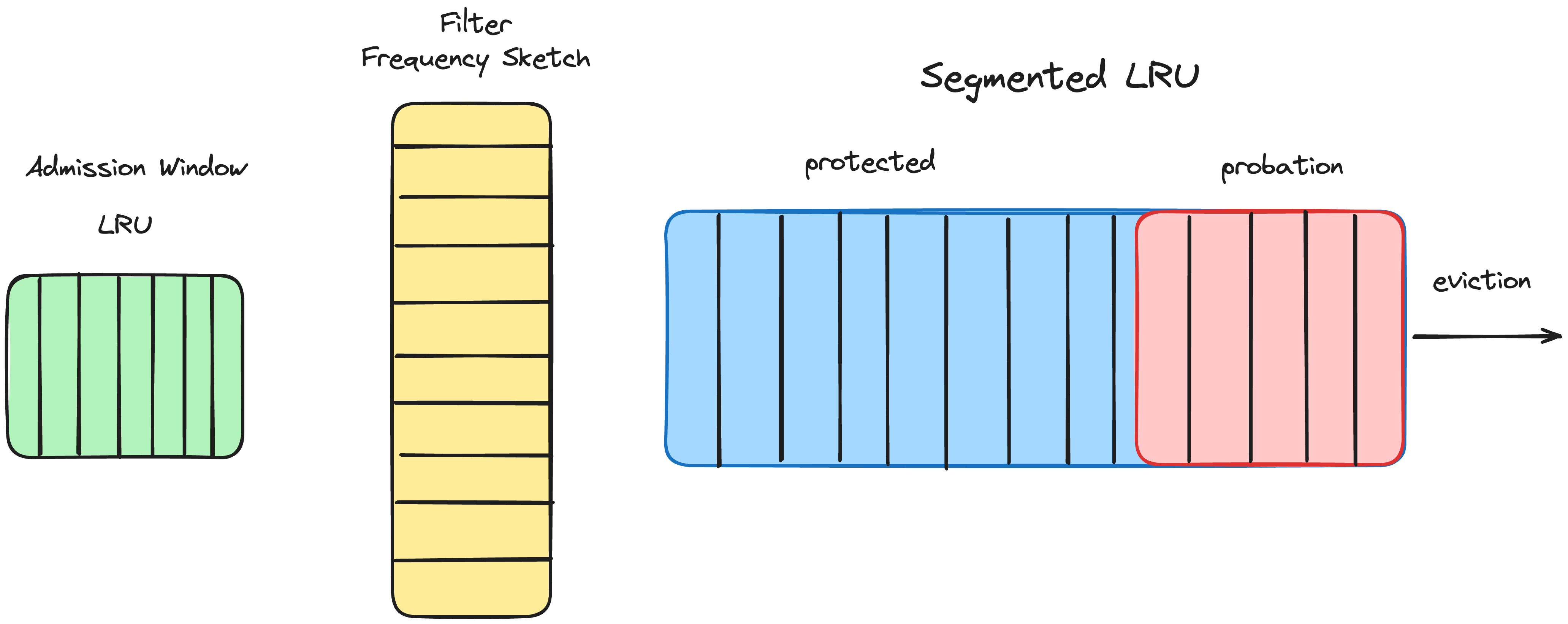
Admission Window: When a new entry is added, it goes through an “admission window” before being fully admitted to the main space. This allows us to have a high hit rate when entries exhibit a bursty access pattern.
Frequency Sketch: Caffeine uses a compact data structure called a CountMinSketch to track the frequency of access for cache entries. This allows it to efficiently estimate the access frequency of the items. If the main space is already full and a new entry needs to be added, Caffeine checks the frequency sketch. It will only admit the new entry if its estimated frequency is higher than the entry that would need to be evicted to make room.

 /**
   * Determines if the candidate should be accepted into the main space, as determined by its
   * frequency relative to the victim. A small amount of randomness is used to protect against hash
   * collision attacks, where the victim's frequency is artificially raised so that no new entries
   * are admitted.
   *
   * @param candidateKey the key for the entry being proposed for long term retention
   * @param victimKey the key for the entry chosen by the eviction policy for replacement
   * @return if the candidate should be admitted and the victim ejected
   */
  @GuardedBy("evictionLock")
  boolean admit(K candidateKey, K victimKey) {
    int victimFreq = frequencySketch().frequency(victimKey);
    int candidateFreq = frequencySketch().frequency(candidateKey);
    if (candidateFreq > victimFreq) {
      return true;
    } else if (candidateFreq >= ADMIT_HASHDOS_THRESHOLD) {
      // The maximum frequency is 15 and halved to 7 after a reset to age the history. An attack
      // exploits that a hot candidate is rejected in favor of a hot victim. The threshold of a warm
      // candidate reduces the number of random acceptances to minimize the impact on the hit rate.
      int random = ThreadLocalRandom.current().nextInt();
      return ((random & 127) == 0);
    }
    return false;
  }

Aging: To keep the cache history fresh, Caffeine periodically “ages” the frequency sketch by halving all the counters. This ensures the cache adapts to changing access patterns over time.
Segmented LRU: For the main space, Caffeine uses a Segmented LRU policy. Entries start in a “probationary” segment, and on subsequent access are promoted to a “protected” segment. When the protected segment is full, entries are evicted back to the probationary segment, where they may eventually be discarded. This is done to ensure that the hottest entries are retained and those that are less often reused become eligible for eviction.

Frequency Sketch

As mentioned, the FrequencySketch class is a key component in the cache’s eviction policy as it provides an efficient way to estimate the popularity (frequency of access) of cache entries. The implementation can be found in the FrequencySketch.java file and is implemented as a 4-bit CountMinSketch. The idea of CountMinSketch is to provide a space-efficient probabilistic data structure for estimating the frequency of items in a data stream. It uses multiple hash functions to map items to a fixed-size array of counters, allowing for a compact representation of frequency information:

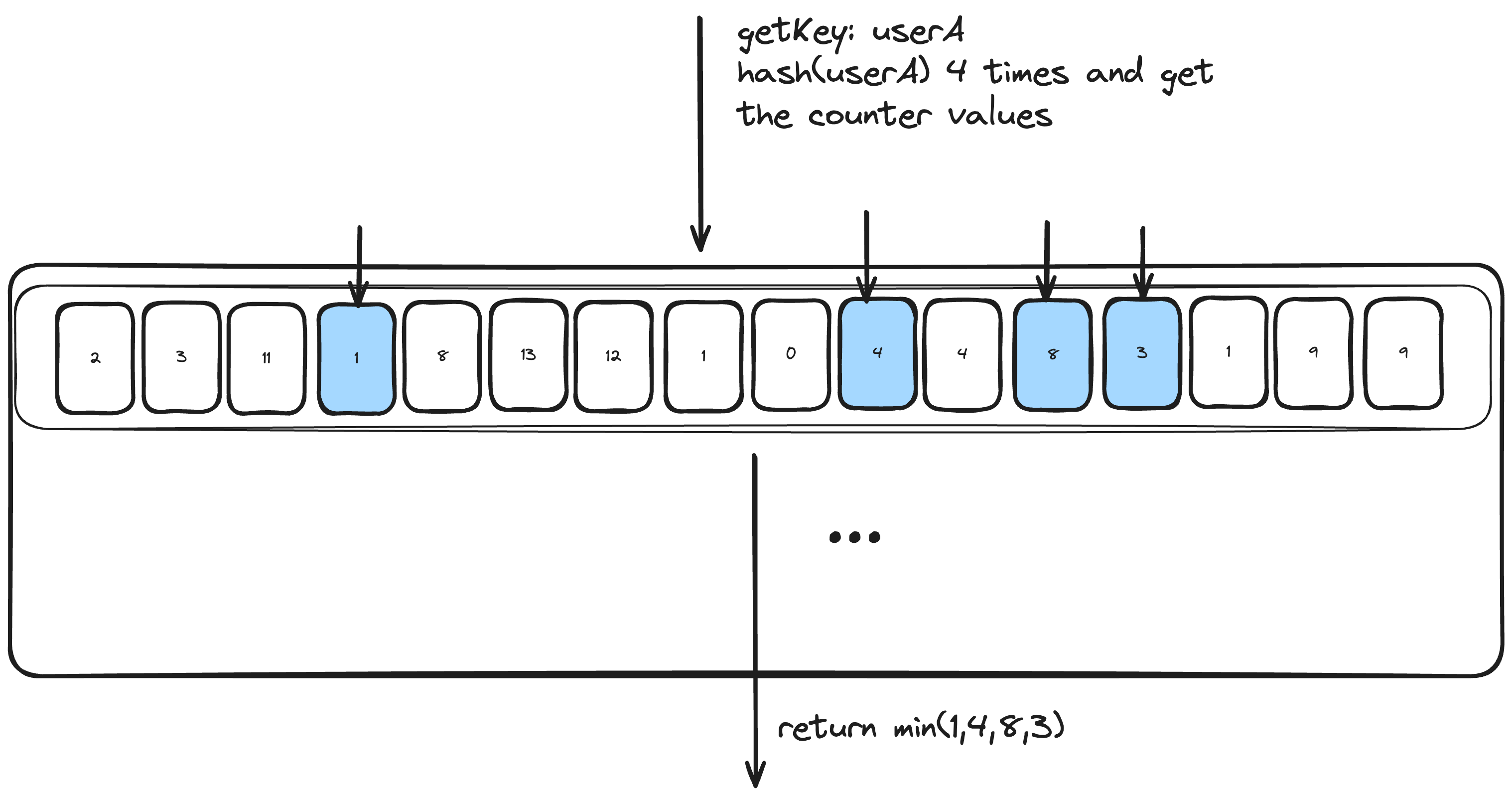
When an item is added or accessed in the cache, it is hashed using multiple hash functions.
Each hash function maps the item to a specific counter in the sketch.
The counters corresponding to the item are incremented.
To estimate an item’s frequency, the minimum value among its corresponding counters is used.

This approach is very clever because it has constant time operations both for updates and queries, regardless of the number of unique items in the cache; it is scalable and memory efficient (it allows to track frequency information with a fixed amount of memory). Let’s look at some interesting bits of its implementation in Caffeine:

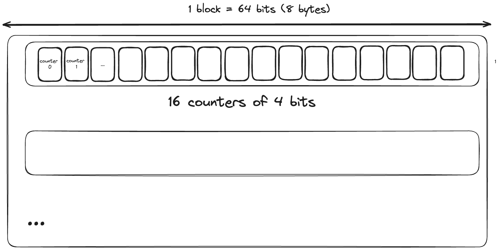
1. Data Structure The sketch itself is represented as a single-dimensional array of 64 bit long values (table). Each long value holds 16 4-bit counters, corresponding to 16 different hash buckets. This layout is chosen to improve efficiency as it keeps the counters for a single entry within a single cache line. Note that the length of the table array is set to the closest power of two greater than or equal to the maximum size of the cache, to enable efficient bit masking operations.

2. Hashing The sketch uses two hashing functions spread() and rehash() to apply supplemental hash functions to the normal element’s hash code.

...
    int blockHash = spread(e.hashCode());
    int counterHash = rehash(blockHash);
...

 /** Applies a supplemental hash function to defend against a poor quality hash. */
  static int spread(int x) {
    x ^= x >>> 17;
    x *= 0xed5ad4bb;
    x ^= x >>> 11;
    x *= 0xac4c1b51;
    x ^= x >>> 15;
    return x;
  }

  /** Applies another round of hashing for additional randomization. */
  static int rehash(int x) {
    x *= 0x31848bab;
    x ^= x >>> 14;
    return x;
  }

3. Frequency Retrieval

The frequency retrieval happens in the method frequency() where it takes the minimum of the 4 relevant counters as a good approximation:

  @NonNegative
  public int frequency(E e) {
    if (isNotInitialized()) {
      return 0;
    }

    int[] count = new int[4];
    int blockHash = spread(e.hashCode());
    int counterHash = rehash(blockHash);
    int block = (blockHash & blockMask) << 3;
    for (int i = 0; i < 4; i++) {
      int h = counterHash >>> (i << 3);
      int index = (h >>> 1) & 15;
      int offset = h & 1;
      count[i] = (int) ((table[block + offset + (i << 1)] >>> (index << 2)) & 0xfL);
    }
    return Math.min(Math.min(count[0], count[1]), Math.min(count[2], count[3]));
  }

The first time I read this I did not understand most of it. It required me to go over a paper and a pencil and do the bit manipulation myself. Moreover, the same happens with the method increment which increments the popularity of an element. Here it is a breakdown of the key steps:

blockHash = spread(e.hashCode()): This spreads the hash code of the input element e to get a better distribution of the hash values.
counterHash = rehash(blockHash): This further rehashes the blockHash to get a different hash value, which will be used to index into the 16 different hash buckets.
int block = (blockHash & blockMask) << 3: To understand this part, we first need to check blockMask and how it is created. It is calculated as (table.length >> 3 ) - 1. The reason why we right-shift the table length by 3 bits is because it is equivalent to divide by 8. Given that each block in the table array contains 16 counters, and each counter is 4 bits wide, the total size of each block is 16*4=64 bits (8 bytes). This means that by right-shifting by 3, we are effectively getting the number of blocks in the table array. We then substract 1 to have all the possible values. For example, if the table length is 256, table.length >> 3 would give us 32; we substract one so it gives us 31, in binary 11111. That includes all the 32 possible values from 0 to 31.

Thus, by masking the blockHash with the blockMask, we ensure that the resulting blocking index is always within the range of the table array.

Then for each iteration (0 to 3), we compute the 4 counter indices:

int h = counterHash >>> (i << 3): This extracts a 8-bit value from the counterHash by right-shifting it by i * 8 bits. This gives us the hash value for the current 4-bit counter.
int index = (h >>> 1) & 15: We first perform a logical right-shift of h by 1 (aka divide by 2) to take the least significant bit. The reason why we do this is to use it later for the offset calculation. We then mask it with 15 (1111 in binary) to get the 4 least significant bits. This gives us the counter index within the block (as there are 16 counters).
int offset = h & 1: This line calculates the offset within the 64-bit block which is either 0 or 1. It does it by taking the least significant bit of the 8-bit hash value.
count[i] = (int) ((table[block + offset + (i << 1)] >>> (index << 2)) & 0xfL): This retrieves the 4-bit counter value from the table by:

Computing the index in the table array where the 4 counters for the given element are located: block + offset + (i << 1):

block is the starting index of the block in the table array
offset is either 0 or 1, depending on which of the two 8-byte segments within the block we are accessing.
(i << 1) is the offset within that 8-byte segment that contains the 4 counters, where i is the counter index (0 to 3). This effectively multiplies i by 2, giving us offsets of 0, 2, 4, or 6 bytes within the 16-byte segment.

Then it righ-shifts this 64-bit value by index * 4 bits with >>> (index << 2). This aligns our 4-bit counter with the least significant bit of the long value. We multiply it by 4 because each counter is 4 bits wide. Then finally, it applies a bitmask to the extracted counter value to ensure that it is a 4-bit unsigned integer & 0xfL (1111 in binary).

Finally, the method returns the minimum value among the 4 frequency counts stored in the count array.

4. Aging Periodically, when the number of observed events reaches a certain threshold (sampleSize) the reset() method is called. This method halves the value of all counters and substract the number of odd counters.

Expiration with Order Queues & Hierarchical TimerWheel

In case we want to understand how things are actually evicted/expired, we must look a bit deeper into the implementation details. For instance, the LRU policies we have seen before in the Segmented LRU and the Admission Window are implemented using an access-order queue, the time-to-live policy (aka eviction based on how long has it been sinde the last write) uses a write-order queue, and the variable expiration uses a hierarchical timer wheel. All of them are implemented efficiently with a O(1) time complexity.

Order queues

Caffeine uses two main queues in the cache that ensure a fast eviction policy. The idea of the queuing policies is to allow for peeking the oldest entry to determine if it has expired. If it has not, then the younger entries must not have expired either. They are both based on the AbstractLinkedDeque.java which provides an optimised double linked list. These are some of the interesting aspects of its implementation:

1. No sentinel nodes

The class uses a double-linked list without sentinel nodes (dummy nodes at the start and the end of the list). As we can see in a comment in the code:

The first and last elements are manipulated instead of a slightly more convenient sentinel element to avoid the insertion of null checks with NullPointerException throws in the byte code. 

this is done to reduce null checks. However, both elements are declared as @Nullable:

@Nullable E first;
@Nullable E last;

so how does it exactly reduce null checks? In a sentinel-based implementation, you always have non-null head and tail nodes. This means you can always safely access head.next and tail.prev without null checks. However, in this implementation without sentinels, first and last can be null. Shouldn’t this require more null checks? The key is in how the JVM handles null checks. When you access a field or method on a potentially null object, the JVM automatically inserts null checks in the bytecode. If the object is null, it throws a NullPointerException. By carefully structuring the code to handle the null cases explicitly, this implementation avoids these automatic null checks and potential NullPointerExceptions in critical paths.

For example, consider the linkFirst method:

void linkFirst(final E e) {
  final E f = first;
  first = e;

  if (f == null) {
    last = e;
  } else {
    setPrevious(f, e);
    setNext(e, f);
  }
  modCount++;
}

This method handles the case where the list is empty (f == null) separately from the case where it’s not. By doing so, it avoids the need for the JVM to insert automatic null checks when accessing fields or methods of f. In a sentinel-based implementation, you might have code like this:

void linkFirst(final E e) {
  Node newNode = new Node(e);
  newNode.next = head.next;
  newNode.prev = head;
  head.next.prev = newNode;  // Potential automatic null check
  head.next = newNode;       // Potential automatic null check
}

Here, the JVM might insert automatic null checks for head.next, even though we know it’s never null.

2. Structural modification tracking

The class maintains an integer modCount to track structural modifications, which is used to detect concurrent modifications during iteration. It is incremented every time an element is added or removed and its primary purpose is to support fail-fast behaviours in iterators:

When an iterator is created, it captures the current modCount:

AbstractLinkedIterator(@Nullable E start) {
  expectedModCount = modCount;
  cursor = start;
}

Every time the iterator perform an operation, it checks if the modCount has changed. If it has changed, it means the list was modified outside of the iterator so it throws an exception:
```
void checkForComodification() {
if (modCount != expectedModCount) {
  throw new ConcurrentModificationException();
}
}
```
The modCount is incremented in methods that structurally modify the list, such as linkFirst(), linkLast(), unlinkFirst(), unlinkLast(), and unlink().

Access Order Queue: AccessOrderDeque.java

The Access Order Queue keeps track of all the entries that are in the hash table based on how recently they were accessed. It is a doubly linked list that maintains the order of cache entries based on access frequency.

When an entry is accessed, it is moved to the tail of the list, ensuring that the least recently used (LRU) entry is always at the head. This is vital for implementing the Least Recently Used (LRU) eviction policy. For example, if we have a cache with entries [A <-> B <-> C] where A is the least recently accessed and C is the most recently accessed, and we access B, it will move it to the end of the queue keeping it like this: [A <-> C <-> B]

Write Order Queue: WriteOrderDeque.java

Similar to the Access Order Queue, the Write Order Queue orders entries based on their creation or update time. It keeps track of the entries based on their write times. This is particularly useful when we want to expire entries after a certain duration since their last write (expireAfterWrite).

For example, consider a scenario where [A <-> B <-> C] are written in that order. If we update A, it will move it to the end of the queue: [B <-> C <-> A].

Hierarchical Timer Wheel: TimerWheel.java

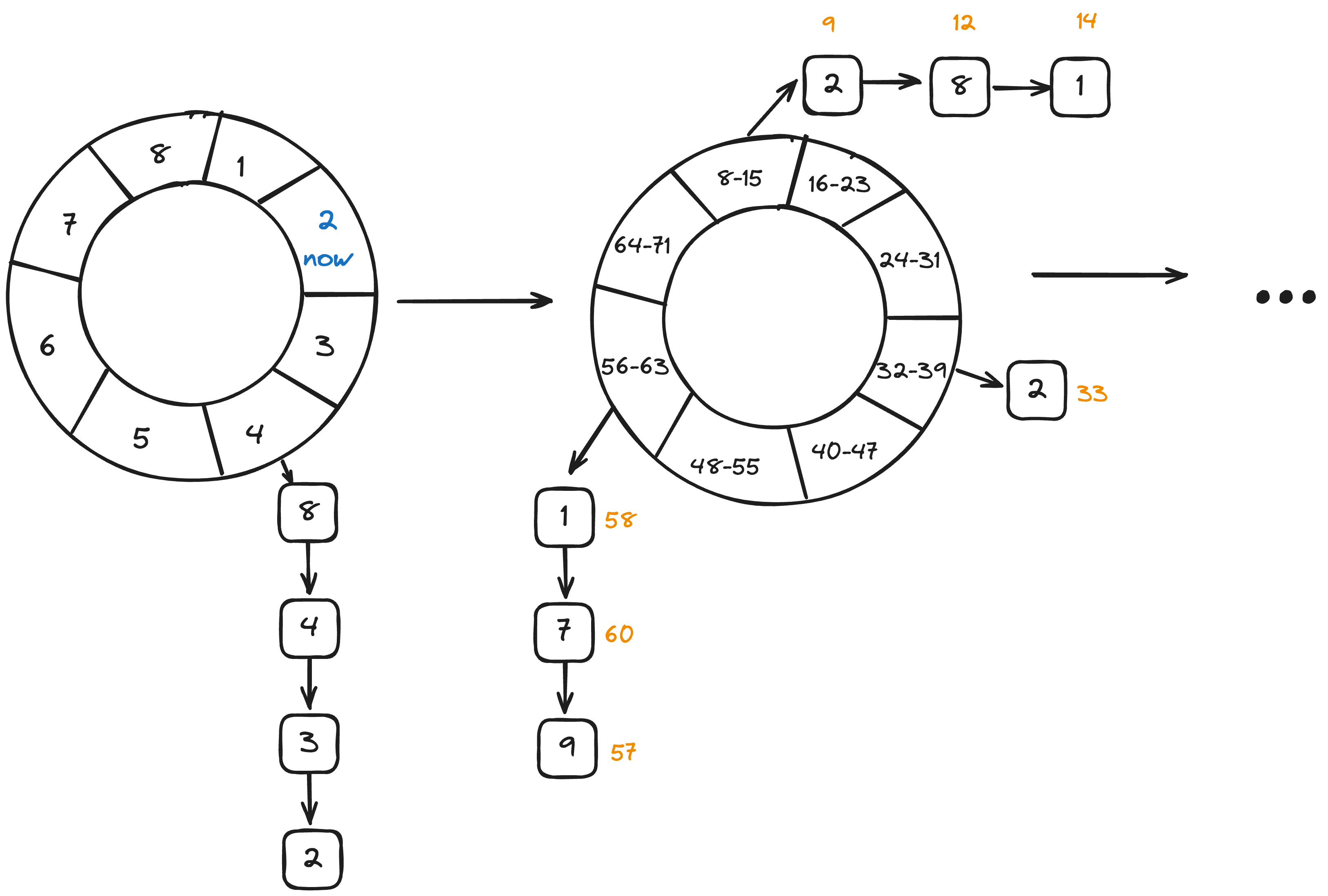
A timer wheel is data structure used to manage time-based events efficiently. The basic idea is that it stores timer events in buckets on a circular buffer, each bucket representing a specific time span (like seconds or minutes).

In the case of Caffeine, the entries are added to these buckets based on their expiration times, allowing efficient addition, removal and expiration in O(1) time. Each bucket contains a linked list where the items are added. Given that the circular buffer size is limited, we would have problems when an event needs to be scheduled for a moment in future larger than the size of the ring. That is why we use a hierarchical timer wheel which simply layers multiple timer wheels with different resolutions.

Let’s take a brief look at the TimerWheel.java code:

1. Hierarchical Structure: Buckets and spans

Each element in the BUCKETS array represents the number of buckets in a timer wheel level, while SPANS defines the duration each bucket covers. As mentioned earlier, the hierarchical structure allows events to cascade from broader to finer time spans. These are the values that were chosen for the Caffeine implementation:

static final int[] BUCKETS = { 64, 64, 32, 4, 1 };
static final long[] SPANS = {
    ceilingPowerOfTwo(TimeUnit.SECONDS.toNanos(1)), // 1.07s
    ceilingPowerOfTwo(TimeUnit.MINUTES.toNanos(1)), // 1.14m
    ceilingPowerOfTwo(TimeUnit.HOURS.toNanos(1)),   // 1.22h
    ceilingPowerOfTwo(TimeUnit.DAYS.toNanos(1)),    // 1.63d
    BUCKETS[3] * ceilingPowerOfTwo(TimeUnit.DAYS.toNanos(1)), // 6.5d
    BUCKETS[3] * ceilingPowerOfTwo(TimeUnit.DAYS.toNanos(1)), // 6.5d
};

2. Clever Bit Manipulation The implementation uses bit manipulation techniques to efficiently calculate bucket indices:

long ticks = (time >>> SHIFT[i]);
int index = (int) (ticks & (wheel[i].length - 1));

This avoids performing expensive modulo operations. Here is a breakdown of how it works:

static final long[] SPANS = {
    ceilingPowerOfTwo(TimeUnit.SECONDS.toNanos(1)), // 1.07s
    ceilingPowerOfTwo(TimeUnit.MINUTES.toNanos(1)), // 1.14m
    // ...
};

static final long[] SHIFT = {
    Long.numberOfTrailingZeros(SPANS[0]),
    Long.numberOfTrailingZeros(SPANS[1]),
    // ...
};

Each SPAN value is rounded up to the nearest power of 2 and the SHIFT array stores the number of trailing zeros for each SPAN value, which is equivalent to $log_2{span[i]}$. It represents the duration of one tick for that wheel. Then, in order to calculate the bucket index we can do some bit manipulation for a very quick calculation of which bucket an event belogs in:

long ticks = (time >>> SHIFT[i]);
int index = (int) (ticks & (wheel[i].length - 1));

time >> SHIFT[i]: this right shifts the appropiate amount for the current wheel, its equivalent to dividing by SPANS[i]
wheel[i].length - 1: this is a bitmask. Since wheel[i].length is always a power of 2, this creates a mask of all 1s in the lower bits.
ticks & (wheel[i].length - 1): this performs a bitwise AND with the mask, which is equivalent to ticks % wheel[i].length but again, much faster.

Let’s look at an example. Suppose we have:

time = 1,500,000,000 nanoseconds (1.5 seconds)
SPANS[i] = 1,073,741,824 (2^30, about 1.07 seconds)
SHIFT[i] = 30

In binary:

time = 1011001010000000000000000000000

Now, when we do time >>> SHIFT[i], we’re shifting right by 30 bits:

1011001010000000000000000000000 >>> 30 = 1

This result, 1, means means that 1 full tick of this wheel has elapsed. For the next part, let’s assume that wheel[i].length is 64. In binary:

ticks = 00000000000000000000000000000001
wheel[i].length - 1 = 00000000000000000000000000111111

we perform the bitwise AND:

  00000000000000000000000000000001
& 00000000000000000000000000111111
  --------------------------------
  00000000000000000000000000000001

and the result is 1, so our index is 1. What this means in practice is that the time (1.5 seconds) has causes the wheel to tick once and this tick places the event in the second bucket of the wheel. The beauty of this approach is that it wraps around automatically. If we had 64 ticks, the index would be 0 again, as 64 & 63 = 0. Suppose the next time value is 3.000.000.000 nanoseconds (3 seconds):

3,000,000,000 >>> 30 = 2 (ticks)
2 & 63 = 2 (index)

So this event would go into the third bucket (index 2) of the wheel.

Adaptative Cache Policy

Caffeine takes a dynamic approach to cache management, continuously adjusting its admission window and main space based on workload characteristics. This adaptation is driven by a hill-climbing algorithm, a straightforward optimization technique that seeks to maximize performance.

The hill-climbing method works by making incremental changes and evaluating their impact. In Caffeine’s context, this means altering the cache configuration (e.g., enlarging the window cache size) and comparing the resulting hit ratio to the previous one. If performance improves, the change is continued in the same direction. If not, the direction is reversed.

The challenge lies in determining the optimal step size and frequency. Measuring hit ratios over short periods can be noisy, making it difficult to distinguish between configuration-induced changes and random fluctuations.

After extensive testing, Caffeine’s developers opted for infrequent but relatively large changes. For example, let’s look at the code that performs the adjustments of window size (source: BoundedLocalCache.java):

  /** Calculates the amount to adapt the window by and sets {@link #adjustment()} accordingly. */
  @GuardedBy("evictionLock")
  void determineAdjustment() {
    // check frequency sketch is initalized
    if (frequencySketch().isNotInitialized()) {
      setPreviousSampleHitRate(0.0);
      setMissesInSample(0);
      setHitsInSample(0);
      return;
    }

    int requestCount = hitsInSample() + missesInSample();
    if (requestCount < frequencySketch().sampleSize) {
      return;
    }

    double hitRate = (double) hitsInSample() / requestCount;
    double hitRateChange = hitRate - previousSampleHitRate();
    double amount = (hitRateChange >= 0) ? stepSize() : -stepSize();
    double nextStepSize = (Math.abs(hitRateChange) >= HILL_CLIMBER_RESTART_THRESHOLD)
        ? HILL_CLIMBER_STEP_PERCENT * maximum() * (amount >= 0 ? 1 : -1)
        : HILL_CLIMBER_STEP_DECAY_RATE * amount;
    setPreviousSampleHitRate(hitRate);
    setAdjustment((long) amount);
    setStepSize(nextStepSize);
    setMissesInSample(0);
    setHitsInSample(0);
  }

It calculates the hit rate based on the hits and total requets of a sample. It compares the current hit rate with the previous one. It the hit rate has improved (or stayed the same), it uses a positive step size; otherwise negative. If the hit rate change is significant, it calculated a larger step size based on a percentage of the maximum possible. Otherwise, it decays the current step size which reduced the magnitude of the change. Finally it ends up updating the state.

This adaptive policy allows Caffeine to fine-tune its behavior to the specific needs of each application, optimizing performance without requiring manual intervention. It’s a testament to the thoughtful design that makes Caffeine stand out in the world of caching solutions.

Conclusion

While there are other intriguing aspects of Caffeine’s internals, such as separate buffers for reads and writes, automatic metrics, and the simulator, I believe we’ve covered enough to grasp its main concepts and inner workings.

Diving into Caffeine’s codebase was truly a blast - it’s a remarkable piece of engineering. From clever bit manipulations to well-designed data structures, it showcases thoughtful and efficient design at every level.

If you found this interesting, I encourage you to visit the repository and give it a star. Ben Manes has created something genuinely impressive here, and it’s worth acknowledging. Hope you learned something valuable from this exploration. High-performance caching might not be glamorous, but it’s a crucial part of many systems, and Caffeine shows how it can be done right.