Today I wanted to talk about the scientific notes with (in my opinion) the funniest name ever: How Often Should You Beat Your Kids? by Don Zagier. Do not worry, it is not what it seems. Even though the paper states facts like the following:

A result is proved which shows, roughly speaking, that one should beat one’s kids every day except Sunday.

it is a joyful text with very cool mathematical tricks (check the sources below if you want to give it a read). However, the paper itself is a continuation of another note: How to Beat Your Kids at Their Own Game by K. Levasseur, another beautiful name for a research text if you ask me. So I guess that first I have to explain this one… So, no rushes… I’ll catch up with Zagier’s work another day. Today let’s dissect the paper with more details on each step.

A Mathematician’s Guide to Outsmarting Children

In How to Beat Your Kids at Their Own Game, the author proposes a simple card-guessing game:

Take a deck with $n$ red cards and $n$ black cards
Turn up cards one at a time
Before each card is revealed, try to predict its color
Keep playing until the deck is empty
Your score is the number of correct guesses

Your opponent’s strategy will be to guess red or black with 50-50 probability each time. On average, yielding $n$ correct guesses (half the deck). However, your optimal strategy will require using a more interesting approach:

Whenever the remaining red and black cards are equal in number, guess randomly.
Otherwise, guess the color that is in the majority.

Surprisingly this leads to an average expected score of:

\begin{equation} n + \frac{\sqrt{\pi n - 1}}{2} + O(n^{-\frac{1}{2}}) \end{equation}

Which, for large $n$, is a major improvement as the term $\frac{\sqrt{\pi n - 1}}{2}$ can be significant. So in other words, you will systematically do better than the kid by harnessing the power of combinatorics. Cool isn’it?

But how do we arrive at that mysteriously precise formula? Let’s break it down into bite-sized pieces!

Breaking Down the Math

Viewing each game as a path

Each game of “Red or black” can be viewed as decreasing path through a grid starting at $(n,n)$ and ending at (0,0).

The x-axis represents how many red cards remain
The y-axis represents how many black cards remain
Each card drawn corresponds to a step left (red) or down (black) until we go from $(n,n)$ to $(0,0)$.

A game is any of those possible paths: sequences of $n$ red and $n$ black cards in some order. There are $\binom{2n}{n}$ such sequences, each equally likely if the deck is shuffled randomly.

Scoring by Counting Diagonal Crossings

To compute the expected score, we need to notice that there are two possibilities:

When red and black counts are equal, your guess is random, yielding an expected $\frac{1}{2}$ points score (because we have the same probability to get a black or a red card).
When one color is in the majority, you guess that color until the counts become equal again.

The key observation here is that your advantage accumulates each time you land on or cross the diagonal (i.e., the line red = black).

Example: If the path visits the diagonal $5$ times, each diagonal crossing gives you an extra $0.5$ “boost” in expected value. So if there are $26$ of each color (a total of $52$ cards), and you cross the diagonal $5$ times, you’d score roughly $26 + (0.5)\times 5 = 28.5$.

In general, if a path visits the diagonal v(p) times in total, the expected score on that path is: \begin{equation} n + 0.5 \times (v(p) -1), \end{equation} where $n$ is the baseline (the kid’s average score) and $v(p) -1$ is how many extra times you guess randomly in the diagonal. Note that we consider visiting $(0,0)$ a diagonal visit; hence the $-1$ in this formula.

The Sum of All Diagonal Visits

To find the expected score, we need the average number of diagonal visits:

Let $P$ be the set of all possible game paths. Since a game path is determined by the $n$ positions of the red cards in a $2n$ card deck, there are $C(2n,n)$ different game paths, being $C$ the combinatoria formula $C(n,x)=\frac{n !}{x !(n-x) !}$.

This holds because we need to choose which $n$ positions out of the $2n$ total draws will be red cards. This is equivalent to choosing $n$ items from $2n$ items, which is what $C(2n,n)$ calculates. For example, if $n=2$, we have $C(4,2) = 6$ possible paths

For any given path $p$, we define $v(p)$ as the number of times the path crosses the diagonal. Given $v(p)$, the expected score is $n + 0.5 \times (v(p)-1)$.

Since we assume a deck of cards randomly shuffled, each of the $C(2n, n)$ paths is equally likely, we can define the expected score $S$ as:

$\begin{aligned} S(n) &=\frac{\sum\limits_{p \in P}(n+0.5 \cdot (v(p)-1))}{C(2 n, n)} \end{aligned}$
$\begin{aligned} S(n) = \frac{\sum\limits_{p \in P} n + \sum\limits_{p \in P} 0.5 \cdot (v(p)-1)}{C(2n, n)} \end{aligned}$
since $n$ is constant across all paths, we can factor it out:
$\begin{aligned} S(n) = \frac{n \cdot C(2n, n) + 0.5 \sum\limits_{p \in P} (v(p)-1)}{C(2n, n)} \end{aligned}$

$\begin{aligned} &= n+0.5\left(\left(\frac{\sum\limits_{p \in P} v(p)}{C(2 n, n)}\right)-1\right) \end{aligned}$

To calculate the total number of times that we visit the diagonal by all game paths, $V(n)$, we define first $\chi(p, m)$ to be $1$ if $p$ visits $(m,m)$ and $0$ otherwise.

$ V(n) =\sum_{p \in P}\left[\sum_{m=0}^{n} \chi(p, m)\right]=\sum_{m=0}^{n}\left[\sum_{p \in P} \chi(p, m)\right]$
$=\sum_{m=0}^{n}$ the number of paths that visit $(m, m)$

To carry on with the proof, we do the following reasoning: If $p$ visits $(m,m)$, then the first $2(n-m)$ cards in the deck are $n-m$ red cards and $n-m$ black cards. Those cards can be rearranged in $C(2(n-m),n-m)$ ways. Also, the other $2m$ cards remaining can be rearranged in $C(2m,m)$ ways. So the total number of game paths that visit $(m,m)$ is

\begin{equation} C(2m,m) \cdot C(2(n-m), n-m) \end{equation}

Therefore

$V(n) = \sum\limits_{m=0}^{n}$ the number of paths that visit $(m, m) = \sum\limits_{m=0}^{n} C(2 m, m) \cdot C(2(n-m), n-m)$

Reminder of geometric series

In order to continue, we need to make a small reminder of geometric series as it will be important to get to the final result.

If A is a sequence of numbers, the generating function of A is $G(A;z) = A(0)+A(1)z+A(2)z^2+A(3)z^3+…=\sum\limits_{n=0}^\infty A(n)z^n$

In our case, the A function that we will use is $A(n)=ar^n$. Hence, its associated generating function is $G(A;z) = \frac{a}{(1-rz)}$ because of the properties of geometric series. Proof:

For $r\neq 1$, the sum of the first n terms corresponds to

$a+ar+ar^2+...+ar^{n-1} = \sum\limits_{k=0}^{n-1}ar^k = a\left( \frac{1-r^n}{1-r}\right)$

In the last two steps, the procedure followed is the next one:

$s =a+a r+a r^{2}+a r^{3}+\cdots+a r^{n-1}$
$r s =a r+a r^{2}+a r^{3}+\cdots+a r^{n-1}+a r^{n}$
we substract them $s-r s =a-a r^{n}$
$s(1-r) =a\left(1-r^{n}\right)$
$s =a\left(\frac{1-r^{n}}{1-r}\right) \quad(\text { if } r \neq 1)$

The case that involves us is when n goes to infinity and r must follow $\mid r \mid<1$ for the serie to converge. Once we establish this conditions, the result of the sum is

\begin{equation} \sum_{k=0}^{\infty}ar^k = \frac{a}{1-r} \end{equation}

because $1-r^n=1$ when $\mid r \mid<1$ and $n\rightarrow \infty$.

Other important properties that will be handy later are that if $A$ and $B$ are sequences of numbers:

\begin{equation} (A\cdot B)(n) = \sum_{m=0}^n A(m) \cdot B(n-m) \end{equation}

and

\begin{equation} G(A\cdot B;z) = G(A;z) \cdot G(B;z) \end{equation}

🧙🏼‍♂️🧙🏼‍♂️ Taylor series magics

Now that all the theory is done, we can follow with this magical statement: Let $V$ be the total number of diagonal visits by all game paths in $P$. Then

\begin{equation} G(V;z) = 1/(1-4z) \Rightarrow V(n) = 4^n \end{equation}

Yeah yeah, I know, this seems to come a bit out of nowhere. To understand this, we need to know that the Taylor series expansion of $1/\sqrt{1-4z}$ is $\sum\limits_{n=0}^{\infty}C(2n,n)z^n$. This identity appears frequently in combinatorics and probability theory. For the proof, instead of differentiating directly (which gets messy), we start with the known binomial series expansion, which itself is derived from Taylor series.

\begin{equation} (1 - x)^{-\alpha} = \sum_{n=0}^{\infty} \frac{\Gamma(\alpha + n)}{\Gamma(\alpha) n!} x^n, \quad \text{for} \quad |x| < 1. \end{equation}

For square roots, we set $\alpha = \frac{1}{2}$: \begin{equation} (1 - x)^{-1/2} = \sum_{n=0}^{\infty} \frac{\Gamma(n + 1/2)}{\Gamma(1/2) n!} x^n. \end{equation}

We know that $\Gamma(1/2) = \sqrt{\pi}$ and also: \begin{equation} \Gamma(n + 1/2) = \frac{(2n)!}{4^n n! \sqrt{\pi}}. \end{equation}

so substituting this into the binomial series: \begin{equation} (1 - x)^{-1/2} = \sum_{n=0}^{\infty} \frac{(2n)!}{4^n (n!)^2 \sqrt{\pi}} \cdot \frac{\sqrt{\pi}}{1} x^n. \end{equation}

Canceling $\sqrt{\pi}$: \begin{equation} (1 - x)^{-1/2} = \sum_{n=0}^{\infty} \frac{(2n)!}{(n!)^2} \frac{x^n}{4^n}. \end{equation}

We can now substitute $x=4x$ into the expansion: \begin{equation} (1 - 4z)^{-1/2} = \sum_{n=0}^{\infty} \frac{(2n)!}{(n!)^2} \frac{(4z)^n}{4^n}. \end{equation}

Since the factors ( 4^n ) in the numerator and denominator cancel out, we obtain: \begin{equation} \frac{1}{\sqrt{1 - 4z}} = \sum_{n=0}^{\infty} \frac{(2n)!}{(n!)^2} z^n. \end{equation}

which is exactly: \begin{equation} \sum_{n=0}^{\infty} C(2n, n) z^n. \end{equation}

So, let $D(n) = C(2n,n)$ and using the geometric series theory above, $V(n) = (D\cdot D)(n)$ so $V = D\cdot D$. And then,

\begin{equation} G(V;z) = G(D\cdot D; z) = G(D;z)^2 = 1/(1-4z) \end{equation}

In this case, the only sequence with this generating function is the geometric sequence $4^n$ therefore, $V(n) = 4^n$.

Wrapping up

\begin{equation} S(n) = n + 0.5 \left( \frac{4^n}{C(2n, n)} - 1 \right). \end{equation}

The first term of this expression represents the portion of the expected score that we would expect from making random guesses, while the second term represents the advantage from counting cards. Given that the second term is difficult to calculate, in the paper they used an asymptotic estimation.

Recall that if $f$, $g$, and $h$ are sequences of real numbers, then $f(n) = g(n) + O(h(n))$ means that there exist integer $N$ and real number $C$ such that $f(n) - g(n) \leq C h(n) $ for all $n \geq N$. If $\lim\limits_{n\to\infty} h(n) = 0$, then $g(n)$ can be used as an approximation of $f(n)$. Of course, the usefulness of the approximation depends on $N$ and $C$.

The used estimation of $S(n)$ is based on Stirling’s approximation of $n!$,

\begin{equation} n! = \sqrt{2\pi n} \left( \frac{n}{e} \right)^n + O\left( \sqrt{\frac{2\pi}{n}} \left( \frac{n}{e} \right)^n \right) \end{equation}

To substitute Stirling’s approximation into $S(n)$, we start with the binomial coefficient: \begin{equation} C(2n, n) = \frac{(2n)!}{(n!)^2}. \end{equation}

and using Stirling’s approximation: \begin{equation} (2n)! \approx \sqrt{4\pi n} \left( \frac{2n}{e} \right)^{2n}, \quad (n!)^2 \approx 2\pi n \left( \frac{n}{e} \right)^{2n}. \end{equation}

Thus, \begin{equation} C(2n, n) \approx \frac{\sqrt{4\pi n} \left( \frac{2n}{e} \right)^{2n}}{(2\pi n) \left( \frac{n}{e} \right)^{2n}} \end{equation}

Simplifying \begin{equation} C(2n, n) \approx \frac{4^n}{\sqrt{\pi n}}. \end{equation}

Substituting the equation: \begin{equation} \frac{4^n}{\binom{2n}{n}} \approx \sqrt{\pi n}, \quad S(n) = n + 0.5 \left(\sqrt{\pi n} - 1\right) + O\left(\frac{1}{\sqrt{n}}\right). \end{equation}

Since $\lim\limits_{n \to \infty} \frac{1}{\sqrt{n}} = 0$, we obtain the final approximation: \begin{equation} S(n) \approx n + 0.5 \sqrt{\pi n} \end{equation}

How accurate is this?

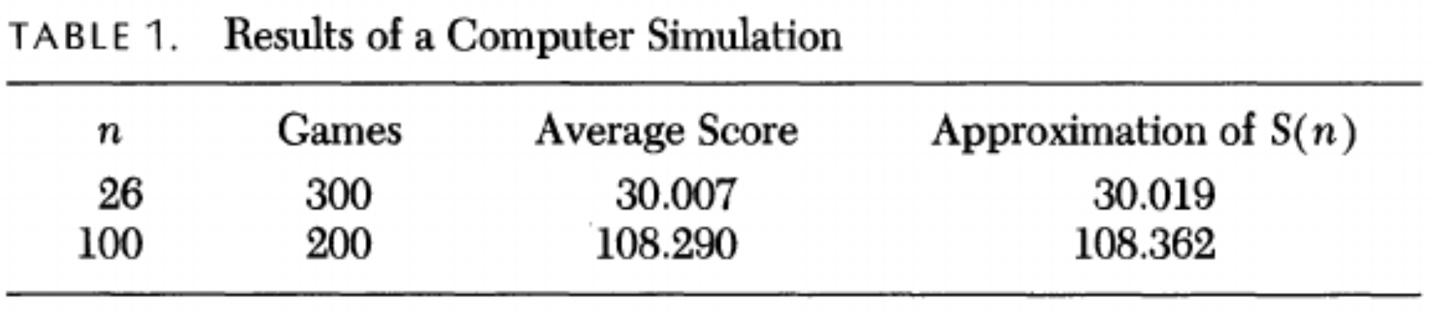
In the paper, they ran a computer simulation using two different values of $n$ ($n=26$ and $n=100$):

Given that the computational power has greatly improved since 1988 (when the paper was written), I took the liberty of generating a more exhaustive simulation:

$n$ from $0$ to $5000$
step size of $10$
for each $n$, run “optimal strategy” $1000$ times

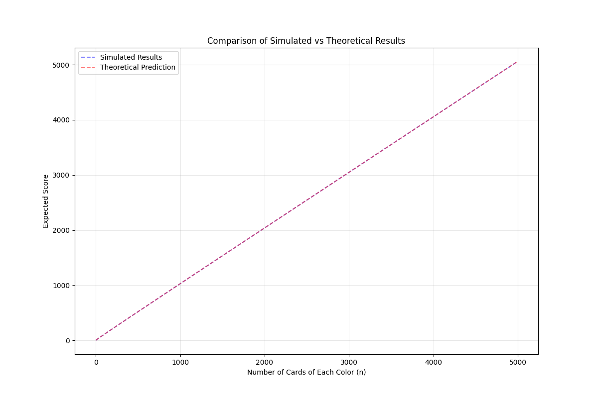
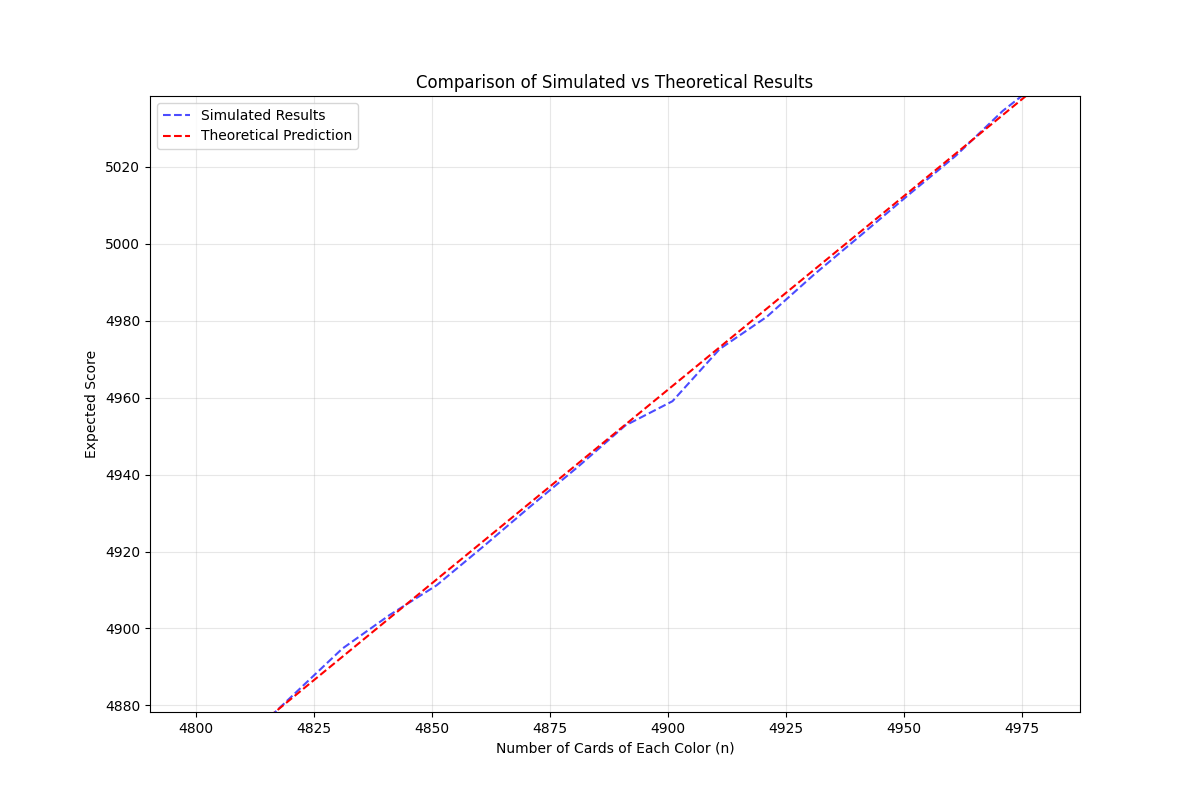
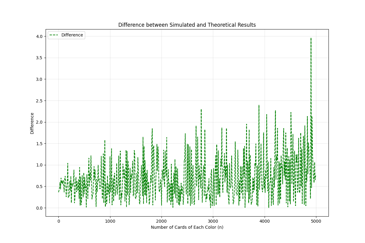
and I was able to check that the estimation is pretty good. You cannot even see the difference in the first figure! That is why I also plotted the difference:

In case you are curious (or you want to play with it), feel free to use the code (disclaimer: this was just a quick script, it is not optimized at all):

import numpy as np
import matplotlib.pyplot as plt

from tqdm import tqdm

def optimal_strategy(n_red: int, n_black: int) -> int:
    total_cards = n_red + n_black
    deck = np.array([0] * n_black + [1] * n_red)
    np.random.shuffle(deck)
    
    score = 0
    remaining_red = n_red
    remaining_black = n_black

    for card in deck:
        if remaining_red == remaining_black:
            guess = np.random.randint(0, 2)
        else:
            guess = 1 if remaining_red > remaining_black else 0
        if card == guess:
            score += 1
        
        remaining_red -= card
        remaining_black -= 1 - card 
    return score
    
    

def theoretical_estimation(n: int) -> float:
    return n + 0.5 * np.sqrt(np.pi * n)

def run_simulation(n: int, num_trials: int) -> (float, float):
    scores = np.array([optimal_strategy(n, n) for _ in range(num_trials)])
    average_score = np.mean(scores)
    expected_score = theoretical_estimation(n)
    return average_score, expected_score

def plot_results(max_n: int, step: int, num_trials: int) -> None:
    ns = range(1, max_n + 1, step)
    simulated_scores = []
    theoretical_scores = []
    
    for n in tqdm(ns, desc="Calculating for different n"):
        avg_score, expected_score = run_simulation(n, num_trials)
        simulated_scores.append(avg_score)
        theoretical_scores.append(expected_score)
    
    plt.figure(figsize=(12, 8))
    plt.plot(ns, simulated_scores, 'b--', label='Simulated Results', alpha=0.5)
    plt.plot(ns, theoretical_scores, 'r--', label='Theoretical Prediction', alpha=0.5)
    plt.xlabel('Number of Cards of Each Color (n)')
    plt.ylabel('Expected Score')
    plt.title('Comparison of Simulated vs Theoretical Results')
    plt.legend()
    plt.grid(True, alpha=0.3)
    plt.show()

    plt.figure(figsize=(12, 8))
    plt.plot(ns, np.abs(np.array(simulated_scores) - np.array(theoretical_scores)), 'g--', label='Difference')
    plt.xlabel('Number of Cards of Each Color (n)')
    plt.ylabel('Difference')
    plt.title('Difference between Simulated and Theoretical Results')
    plt.legend()
    plt.grid(True, alpha=0.3)
    plt.show()
    
    print("\nDetailed results for n=26 (standard deck size):")
    avg_26, expected_26 = run_simulation(26, num_trials=1_000)
    print(f"Simulated average score: {avg_26:.2f}")
    print(f"Theoretical expected score: {expected_26:.2f}")
    print(f"Difference: {abs(avg_26 - expected_26):.2f}")
    

    print("\nDetailed results for n=100:")
    avg_100, expected_100 = run_simulation(100, num_trials=1_000)
    print(f"Simulated average score: {avg_100:.2f}")
    print(f"Theoretical expected score: {expected_100:.2f}")
    print(f"Difference: {abs(avg_100 - expected_100):.2f}")

if __name__ == "__main__":
    np.random.seed(42)
    plot_results(max_n=5_000, step=10, num_trials=1_000)

Output of the script:

> python computation.py
Detailed results for n=26 (standard deck size):
Simulated average score: 29.88
Theoretical expected score: 30.52
Difference: 0.64

Detailed results for n=100:
Simulated average score: 108.39
Theoretical expected score: 108.86
Difference: 0.48