Efficiently perform Approximate Nearest Neighbor Search at Scale
At Datadog, we regularly hold hackathons, a dedicated time when we can explore new ideas and tinker with new technologies. During one of these hackathons, I found myself working side by side with a colleague who holds a Data Mining & Algorithms PhD. Driven by the desire to do something both cool and complex, we decided on building an online anomaly detection method for streaming logs. We both work in the Cloud SIEM team, a team that provides a security tool to analyse logs in a stateful manner so we were not starting from scratch and we had most of the building blocks to make it in a limited amount of time.
Before getting into implementation, we spent a whole day exploring ideas and options, existing papers and blog posts on a range of topics from efficient data representation and data structures, to online clustering and approximate nearest neighbor search algorithms. One approach that striked as a heavy contestant was SPANN, which stands for Simple yet efficient Partioning-based Approximate Nearest Neighbour, a pretty cool algorithm introduced by Microsoft Research to perform approximate nearest neighbour searches. I originally discovered it via a turbopuffer post in hackernews (for the ones who don’t know about turbopuffer, it is a vector database that leverages object storage as its persistent layer), and its core idea is to keep only cluster centroids (representatives of groups of points) in memory, and store the actual points on disk. This ensures lower memory usage when the dataset scales to massive volumes, which is particularly valuable in large-scale vector search scenarios like web search.
Even though we did not end up pursuing SPANN for the hackathon, eventually, my curiosity led me to read the SPANN (and SPFresh, which is basically an improvement in case you need efficient index updates) paper. Impressed by the brilliance of it, and having (for the longest time) a long-standing intention to learn Rust, I decided to implement a flavor of the SPANN algorithm myself, partly as a learning exercise on SPANN’s ideas and partly to gain hands-on experience with Rust’s development workflow.
The result of that experiment is adriANN, a small toy Rust crate full of newbie mistakes (oopsie). However, I can confirm that the core ideas and tricks of SPANN stayed with me (you get a whole new level of knowledge when you have to implement it yourself). So below, I’ll walk through the main ideas behind SPANN, demonstrating how a memory-efficient, hybrid ANN search can yield high recall and low latency. Moreover, we will see why this method makes a lot of sense when trying to implement an object-storage backed nearest neighbour search (just like turbopuffer did). If I find the time, I might end up writing a second part on SPFresh.
SPANN 101
Vector search is used for a lot of different high-scale applications: from Pinterest’s discovery feature to personalized recommendations on Amazon. The main challenge of modern vector search is to process billions of vectors with minimal latency at a reasonable cost. Storing all these vectors in memory can be incredibly expensive and sometimes not feasible. SPANN’s algorithm addresses this challenge by:
-
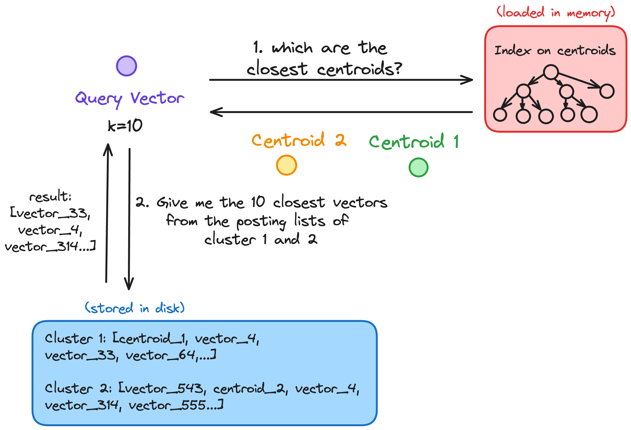
Splitting Data between Memory and Disk Instead of holding every data point in memory, SPANN only stores cluster centroids (representative points) of groups. The remaining points (often billions of them) reside on disk. This drastically cuts down on memory usage, making it more practical to handle web-scale data. The idea is based on performing an initial blazingly fast search on an index that only contains those representative points. Once we have the representatives, we can load the posting lists that are most relevant to a query, load those from disk, and perform a more detailed similarity search. Because the posting lists are well-clustered, the recall remains high, while the disk loads remain minima.
-
Efficient Disk Access: Because the actual vectors live on disk, disk I/O could become a bottleneck. SPANN tries to mitigate that bottleneck as much as possible by using a balanced clustering algorithm. That ensures that the number of points you need to load from disk for a query remains small.
** SPANN Tricks: the cool stuff**
The core idea of splitting the stuff into memory and disk is quite neat but easy to understand. The really cool stuff comes when you explore the different tricks that SPANN came up with to really exploit that advantage.
How the Memory Index Is Constructed?
As mentioned earlier, the memory index holds the centroids of the dataset, representatives of their partition. So in order to build that index, we need to first find the centroids. This is especially important because to support fast lookups and keep disk access efficient, the quality of the centroids really matters.
Think of it like this: we want to split our dataset into lots of small, well-sized chunks. The final result of these chunks is a posting list which stores the list of the points that live in that certain region of space.
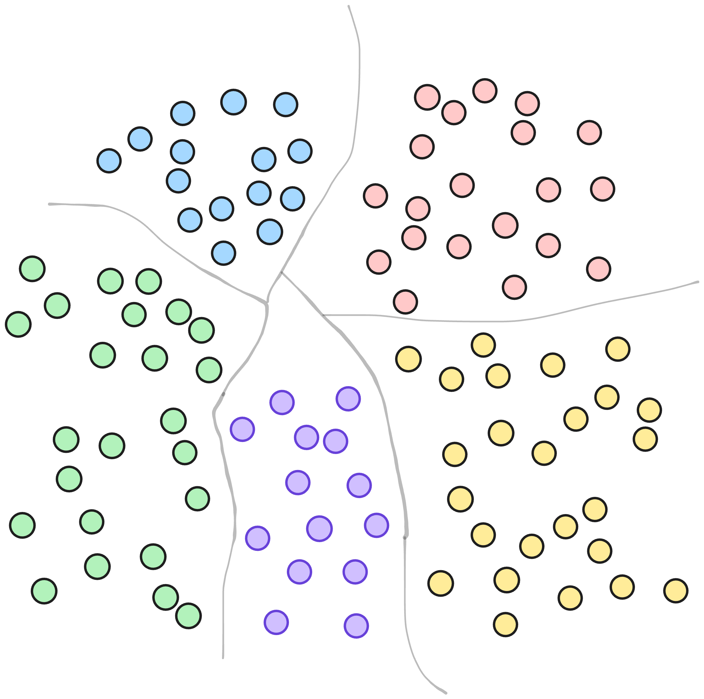
There are several methods to do that, in the case of SPANN, we use a hierarchical balanced clustering method. The reason behind this decision is because imbalance kills performance and the algorithm ensures well balanced clusters. Imagine you have a posting list with 100 vectors and another with 100,000, your I/O pattern would become unpredictable and your latency would spike. Moreover retrieving a big posting list would mean a lot of time spent loading data from disk.
But partitioning a huge dataset isn’t simple. When you’re clustering millions of vectors, normal k-means (or even fancier constrained clustering algorithms) just can’t keep up. That’s where hierarchical clustering steps in. Instead of trying to split the data into N pieces all at once (which is slow and expensive), SPANN does it in stages:
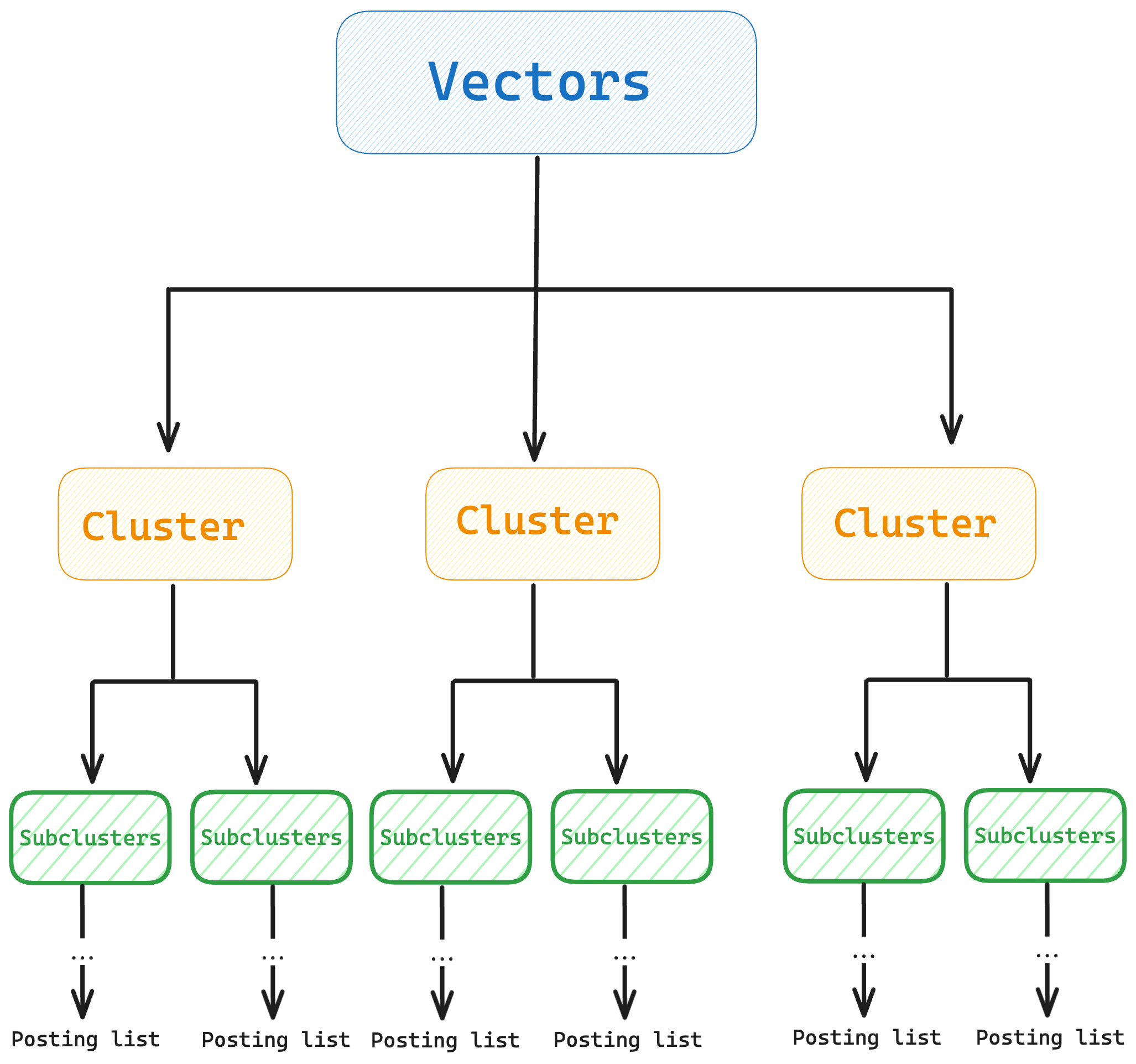
- First, split the data into a small number of clusters—say, k. You can use basic k-means for this.
- Then, take each of those clusters and split them again into k sub-clusters.
- Keep repeating until you’ve got the total number of clusters you need (N). Each final cluster will have a representative (centroid) and will have a posting list including all of its points which will be stored on disk.
Note: In the paper they made extensive experiments to decide which is the best amount of clusters (or centroids) in terms of accuracy and performance. Their conclusion was that 16% of the points as centroids was a good value to achieve both good search performance and small memory usage.
On top of that, SPANN also adds a few smart tricks:
-
Instead of using the centroid (which is just an average point that doesn’t actually exist in your dataset), it picks the real vector that’s closest to the centroid to represent the cluster. This ensures that the “navigational computation” is more meaningful.
-
Once all the posting lists are built, we still need to quickly figure out which ones are relevant to a given query. SPANN solves this by indexing the representative vectors using SPTAG, a hybrid graph/tree structure that makes it super fast to find the nearest ones. In my own project, AdriANN, I was kinda lazy so I used a great KD-tree library called Kiddo instead.
adriANN note. After experimenting with the full hierarchical balanced clustering pipeline (k-means++ init, iterative centroid updates, recursive subdivision, boundary-threshold + RNG duplication), I ended up replacing it with plain random sampling. For real-world datasets, the law of large numbers covers large inputs (a random sample of K points is a representative sample of the underlying distribution), and small inputs are essentially insensitive to minor head-index imbalance. Each point is then assigned to its
Lnearest centroids — that’s it. Recall stays within noise of the more elaborate scheme on GIST1M, and the code got about 500 lines shorter. Seesrc/clustering/random_sample.rsin the repo.
Dealing with Boundary Vectors
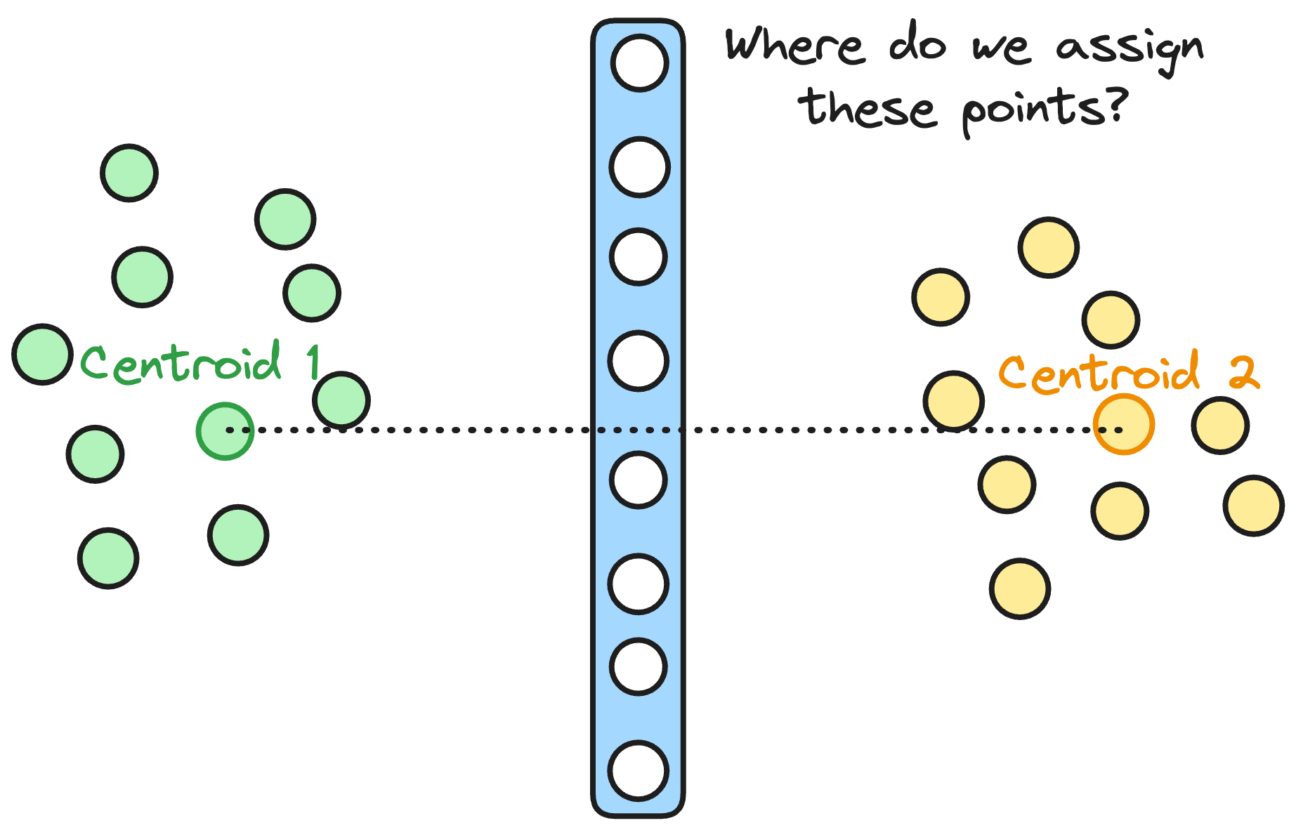
So what happens if you’re a lonely vector exactly on the edge between two clusters? In a perfect world, data splits into clearly defined “territories,” but real-world data is messier. If a vector is near the boundary of multiple centroids, assigning it to just one cluster might hamper recall if the real nearest neighbor lives in a neighboring cluster.
SPANN has a specific strategy to deal with those: Duplicate Only What’s Necessary. One naive fix is to allow a vector to belong to multiple close clusters. This definitely ups your recall potential: no more missed neighbors just because your data drew an imaginary boundary. However, this can blow up very easily and can lead to heavier disk reads due to several clusters containing that boundary vector.
In SPANN, instead of going overboard, we only duplicate the “boundary” vectors whose distances to more than one centroid are almost the same. Vectors that are comfortably closer to one centroid remain single-cluster members.
The paper does this with a threshold (“close enough to multiple centroids”) plus an RNG-style check to skip redundant duplications. adriANN takes a simpler route that produces the same effect: every point is always assigned to its L nearest centroids, full stop. L (the replica_count parameter) is typically 8. Points in the middle of one cluster still get replicated into their 8 nearest neighbors — which is a bit wasteful, but the posting-list overhead is bounded linearly in L and there are no knobs to tune beyond one number.
// From src/clustering/random_sample.rs — per-point top-L assignment:
let point = self.data.row(point_idx);
let mut dists: Vec<(usize, f32)> = centroid_indices
    .iter()
    .enumerate()
    .map(|(cluster_id, &c_idx)| {
        let c_row = self.data.row(c_idx);
        (cluster_id, metric.compute(point_slice, c_row.as_slice().unwrap()))
    })
    .collect();
// Partial sort: the L smallest at the front.
dists.select_nth_unstable_by(l - 1, |a, b| {
    a.1.partial_cmp(&b.1).unwrap_or(std::cmp::Ordering::Greater)
});
for (cluster_id, _) in dists.into_iter().take(l) {
    // Emit (cluster_id, point_idx) — this point joins L posting lists.
}
Relative Neighborhood Graph rule
So now we have boundary vectors assigned to multiple clusters. Great! Unless those clusters are super close to each other. In that case, we risk lots of the same boundary vectors living in both clusters. That means duplicate reads from nearly identical posting lists. Ouch!
To combat this, we add a final check using the Relative Neighborhood Graph (RNG) rule. Put simply, when deciding if we should assign a vector to a second (or third) cluster we check whether the distance between that vector and its centroid is larger than the distance between the vector and the centroid of the cluster you have already chosen. The idea is to avoid storing the same boundary vector in multiple highly similar posting lists. More formally, it would be defined as:
Only assign the vector $x$ to an additional centroid $c2$ if:
being $c1$ the nearest centroid to $x$.
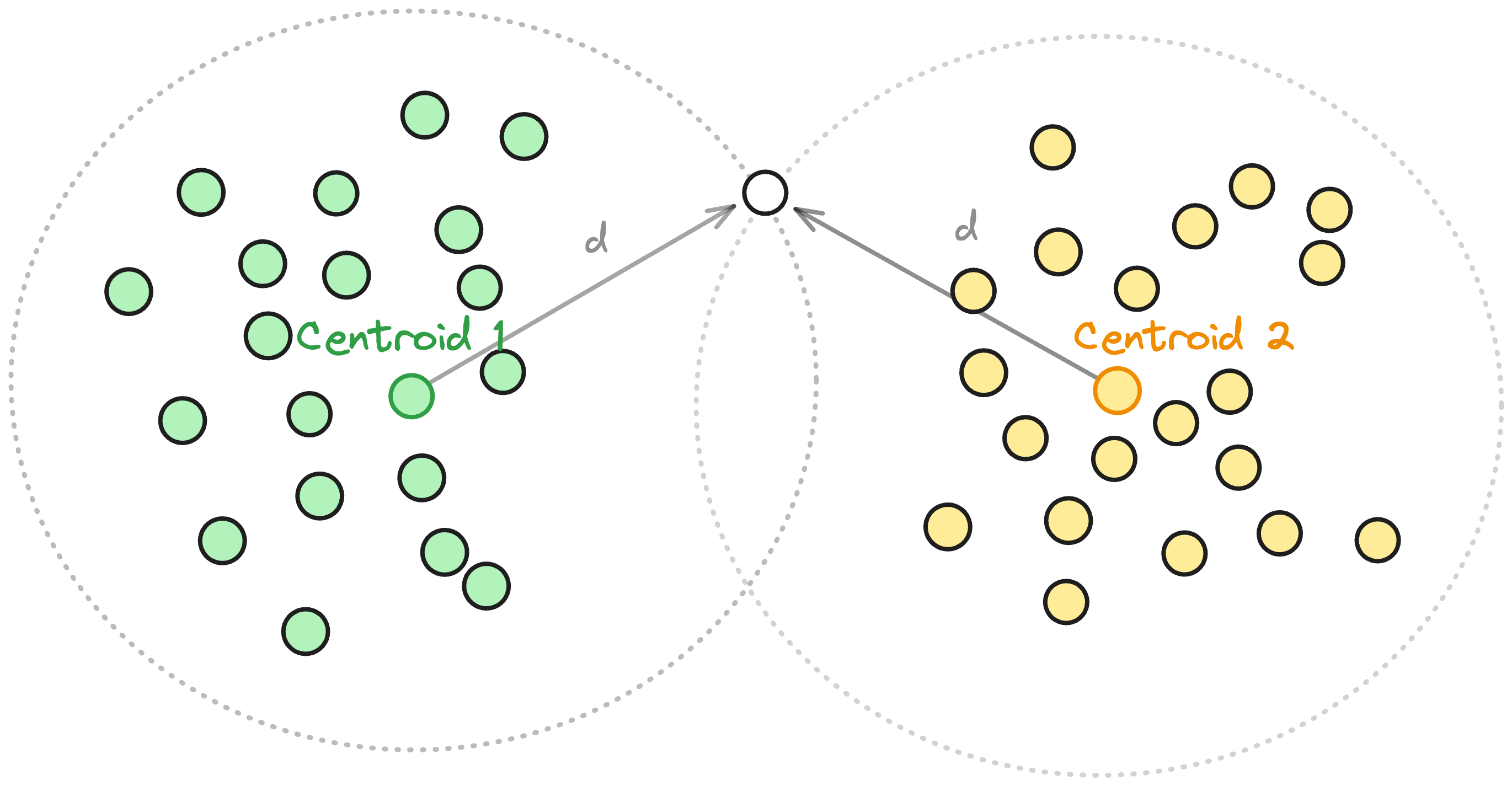
The intuition of this rule is way easier if we imagine it like a Venn Diagrams. Imagine each centroid’s cluster as a circle. A boundary vector x near two overlapping circles might fall into both, but if the circles almost fully overlap, adding x to both lists is redundant so it is not worth to duplicate it. The RNG rule asks: Are these circles overlapping too much to bother duplicating? If yes, skip it.
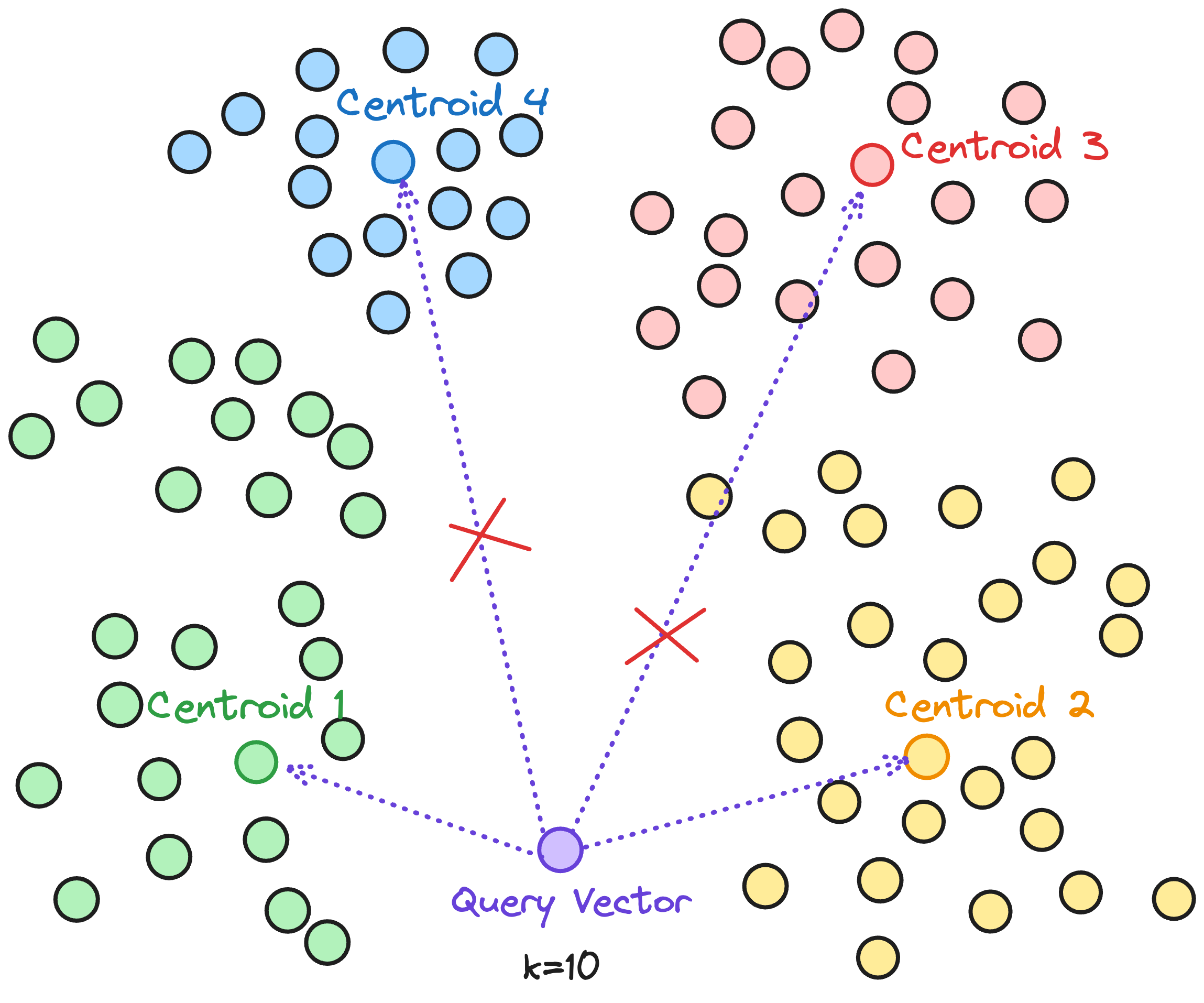
Query-Aware Dynamic Pruning
When it comes to searching vectors at enormous scales, you often can’t afford to go through a lot of clusters, especially if you’re aiming for low-latency responses. A common approach when searching the $K$ nearest neighbors is to grab the $K$ closest centroids and then search within all of them. While this is simpler, it doesn’t exactly scream efficiency. Sometimes the kth closest list is much farther away than the top few. Searching these far-flung lists can be a big waste of time and resources if you don’t expect to find relevant neighbors there anyway.
SPANN, instead of blindly searching all $K$ posting lists, does a mini check to see if a particular posting list’s centroid is truly in the ballpark of the closest centroid. Formally:
Only search posting list $i$ if $Dist(q,c_i)≤(1+γ) \cdot Dist(q,c 1)$ where:
- $q$ is the query vector
- $c_i$ is the centroid of cluster
- $c_1$ is the nearest centroid
- $γ$ is is a small factor (i.e. $0.2$) indicating how tolerant we are of “near-ish” clusters.
Or in plain English, we skip any centroid that’s significantly farther away than the nearest one. This means if the distance between $q$ and $c$ is, say $10$ times bigger than the distance to $c_1$, that cluster isn’t probably worth the time.
// From src/spann/spann_index.rs — current query path:
let nearest_centroids = self.kdtree.nearest_n::<kiddo::SquaredEuclidean>(&q, k);
// SPANN centroid-gating: (1 + gamma) * dist(q, c1)
let threshold = (1.0 + self.gamma) * nearest_centroids[0].distance;

// top_k is a bounded max-heap of size k, so the inner loop is O(points · log k).
for nn in nearest_centroids {
    if nn.distance > threshold { continue; }
    self.posting_list_store.visit(nn.item as usize, |id, v| {
        let dist = metric.compute(query, v);
        if top_k.len() < k {
            top_k.push((id, dist, v));
        } else if dist < top_k.peek_max().dist {
            top_k.replace_max((id, dist, v));
        }
    });
}
A couple of notes on the current implementation:
- The distance metric is configurable (
EuclideanorManhattan) and stored on the index, so both the KD-tree pre-filter and the final ranking use the same metric. An earlier version hard-coded squared-Euclidean at ranking time, which quietly wrecked recall when the user configured Manhattan — now guarded by an end-to-end test. - Posting lists are memory-mapped from disk in a flat
[u32 ids | f32 vectors]layout, so thevisitcallback iterates over&[f32]slices straight out of the mmap — no per-query deserialization. - Inner distance loops use explicit SIMD (
wide::f32x8) and the release profile is built with-C target-cpu=native, so AVX2/AVX-512/NEON get picked up automatically. - A
query_intovariant takes a caller-provided&mut [Option<PointData>]and uses it directly as the heap, letting you amortize allocations across batches.
Why does it make sense to use it for Object-Storage backed-up Nearest Neighbor Search?
As mentioned earlier, I stumbled upon SPANN through the Turbopuffer architecture page, and after reading it, quickly it became clear why they opted for this approach: scalability and costs. Nowadays, there is an increasing number of databases and data-intensive applications that are relying on object storage by design, some examples include:
- WarpStream: A high-performance Kafka replacement that uses S3.
- Neon: A cloud-native Postgres service that separates storage and compute for elastic scaling.
- SlateDB: An embedded lightweight database leveraging object storage as the primary persistence layer.
so it is not surprising to see a vector database taking that approach as well. It is worth noting that there are plenty of other vector databases that are already designed to work on top of Object Storage like Pinecone or Milvus; and each of them has their own approach for indexing. Milvus for example, allows the customer to try different algorithms like IVF or HNSW and Pinecone has its own proprietary algorithm that looks suspiciously similar to SPFresh.
Scalability without sharding/operation nightmares:
If your dataset grows a lot or you want to push updates incrementally, object storage can handle that more gracefully than trying to continuously re-shard or expand a giant in-memory cluster. In traditional in-memory setups, scaling often means introducing complex sharding mechanisms or rebalancing the dataset, both of which can become operational headaches as the dataset grows. With object storage:
- Adding new vectors is as simple as adding objects into a bucket.
- There’s no need for complex re-sharding operations; storage can grow seamlessly.
- You can leverage the inherent scalability and durability of object storage systems.
Challenges
We know that in a system design on top of S3 (for the sake of simplicity let’s imagine that Object/Blob Storage == S3), the most problematic parts are gonna be S3 calls costs and latency.
Minimize S3 calls (aka 💸💸) and latency
Imagine you want to implement SPANN using Blob Storage. You could store the centroids index, and the different posting lists in S3. When the application boots, it would only fetch the index and load it into memory. Then you’d fetch only the necessary posting lists based on the algorithm. Given the characteristics we’ve mentioned before, SPANN will always try to minimize the amount of data we fetch from disk (aka blob storage) so this approach is much more efficient when it comes to minimize roundtrips and calls to S3, compared to the some of the other famous approximate nearest neighbour approaches like HNSW or DiskANN.
This is because SPANN-style algorithms use a two-tiered strategy:
- A compact in-memory index of centroids handles most of the search effort upfront.
- Only a few disk-based posting lists (clusters of actual vectors) need to be fetched on demand.
That drastically reduces unnecessary I/O. In contrast, methods like HNSW typically need to hop between multiple random-access neighbors during a search— a pattern that’s devastating for latency and cost when each access maps to a remote S3 GET.
Content-Aware Routing in Distributed Mode
Each time a query identifies relevant clusters to search (after checking the in memory index), you’ll need to fetch the associated vectors from object storage. To avoid incurring a separate GET call per vector, we could store full posting lists as blobs (or parquet chunks, or whatever suits your tech stack), so that a single S3 GET retrieves a full batch of vectors. On top of that, if you’re deploying this system across multiple nodes (e.g., Kubernetes pods, serverless workers, or even regional replicas), we could make sure to route queries to the right node. This can be done by hashing on customer ID, vector namespace, or some custom sharding key to:
- Maximize the chance of cache hits
- Avoid duplicating S3 reads across nodes
- Simplify index consistency and memory management
This can be particularly helpful in hot-shard workloads where popular centroids get queried frequently.
Preload Popular Centroids and Posting Lists
You’ll likely observe skewed query patterns — e.g., some clusters being hit far more often due to time of day, geography, or tenant distribution. Instead of letting those hit cold storage repeatedly:
- Track hot centroids using a Count-Min Sketch or rolling counters.
- Proactively preload and pin those posting lists into cache, either at startup or on a rolling window.
This behavior mirrors how modern systems like Caffeine handle popularity-based cache promotion.
Final Thoughts
Implementing ANN search on top of object storage might sound like heresy to those used to ultra-low-latency in-memory solutions — but when done right, it offers a compelling blend of scalability, cost-efficiency, and robustness. SPANN and its successors like SPFresh are well-suited to this architecture because they’re inherently disk-friendly and avoid the pointer-chasing behaviors that kill performance on remote storage.
SPANN isn’t just a clever algorithm — it’s a blueprint for rethinking how we structure vector search in modern cloud-native systems. If I find time (and another burst of masochistic curiosity), I’ll follow up with a post exploring SPFresh’s updates-focused improvements and what I learned implementing online indexing in Rust.
Until then, happy hacking — and don’t forget to cache your centroids! 🚀